Real eigenvalues and eigenvectors of 3x3 matrices, example 1

In these examples, the eigenvalues of matrices will turn out to be real values. In other words, the eigenvalues and eigenvectors reside entirely in \(\mathbb{R}^n\).
Suppose we have the following matrix:
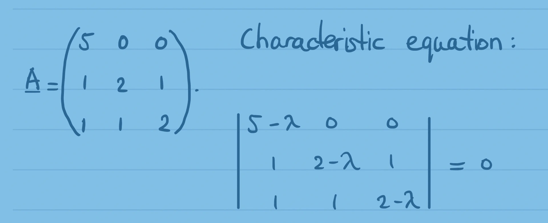
\[\mathbf{A} = \begin{pmatrix} 5 & 0 & 0 \\ 1 & 2 & 1 \\ 1 & 1 & 2 \end{pmatrix}.\]
The objective is to find the eigenvalues and the corresponding eigenvectors.
Characteristic equation
Firstly, formulate the characteristic equation and solve it. The solutions are the eigenvalues of matrix \(\mathbf{A}\).
If \(\mathbf{I}\) is the \(3 \times 3\) identity matrix and \(\lambda\) represents the scalar eigenvalue, the characteristic equation is given by:
\[\det(\mathbf{A} - \lambda \mathbf{I}) = 0.\]
Written in determinant form:
\[\begin{vmatrix} 5-\lambda & 0 & 0 \\ 1 & 2-\lambda & 1 \\ 1 & 1 & 2-\lambda \end{vmatrix} = 0.\]
Choose the row or column easiest to use to compute the determinant. In this case, we expand along the first row because it contains two zeros and only one non-zero entry, \((5-\lambda)\):
\[(5-\lambda) \begin{vmatrix} 2-\lambda & 1 \\ 1 & 2-\lambda \end{vmatrix} - 0 \begin{vmatrix} 1 & 1 \\ 1 & 2-\lambda \end{vmatrix} + 0 \begin{vmatrix} 1 & 2-\lambda \\ 1 & 1 \end{vmatrix} = 0,\]
\[(5-\lambda) \begin{vmatrix} 2-\lambda & 1 \\ 1 & 2-\lambda \end{vmatrix} = 0.\]
Evaluating the \(2 \times 2\) determinant:
\[\begin{aligned} (5-\lambda)\left[(2-\lambda)^2 - 1^2\right] &= 0, \\ (5-\lambda)\left[4 - 4\lambda + \lambda^2 - 1\right] &= 0, \\ (5-\lambda)(\lambda^2 - 4\lambda + 3) &= 0. \end{aligned}\]
Factoring the quadratic term yields:
\[(5-\lambda)(\lambda - 1)(\lambda - 3) = 0.\]
The roots of the characteristic equation are immediately apparent:
\[\lambda = 1 \quad \vee \quad \lambda = 3 \quad \vee \quad \lambda = 5.\]
Verifying the eigenvalues
We can verify these eigenvalues by checking the matrix trace and determinant:
- Trace check: The sum of the eigenvalues must equal the trace of \(\mathbf{A}\) (the sum of the main diagonal elements): \[\text{tr}(\mathbf{A}) = 5 + 2 + 2 = 9 \quad \Longleftrightarrow \quad 1 + 3 + 5 = 9. \quad \checkmark\]
- Determinant check: The product of the eigenvalues must equal \(\det(\mathbf{A})\): \[\det(\mathbf{A}) = 5\left(2^2 - 1^2\right) = 5(3) = 15 \quad \Longleftrightarrow \quad 1 \times 3 \times 5 = 15. \quad \checkmark\]
Eigenvector equations
To determine the eigenvectors, let:
\[\mathbf{v} = \begin{pmatrix} x_1 \\ x_2 \\ x_3 \end{pmatrix},\]
satisfying:
\[(\mathbf{A} - \lambda \mathbf{I})\mathbf{v} = \mathbf{0}.\]
In explicit matrix form:
\[\begin{pmatrix} 5-\lambda & 0 & 0 \\ 1 & 2-\lambda & 1 \\ 1 & 1 & 2-\lambda \end{pmatrix} \begin{pmatrix} x_1 \\ x_2 \\ x_3 \end{pmatrix} = \begin{pmatrix} 0 \\ 0 \\ 0 \end{pmatrix},\]
which gives the following system of linear equations:
\[\begin{cases} (5-\lambda)x_1 = 0, \\ x_1 + (2-\lambda)x_2 + x_3 = 0, \\ x_1 + x_2 + (2-\lambda)x_3 = 0. \end{cases}\]
Finding the eigenvectors
Eigenvalue \(\lambda = 1\)
Substituting \(\lambda = 1\) into the eigenvector equations:
\[\begin{cases} 4x_1 = 0, \\ x_1 + x_2 + x_3 = 0, \\ x_1 + x_2 + x_3 = 0. \end{cases}\]
The first equation gives \(x_1 = 0\). Substituting \(x_1 = 0\) into the remaining equations gives \(x_2 + x_3 = 0\), or \(x_2 = -x_3\). Setting \(x_3 = 1\) yields \(x_2 = -1\).
Thus, an eigenvector corresponding to \(\lambda = 1\) is:
\[\mathbf{v}_1 = \begin{pmatrix} \phantom{-}0 \\ -1 \\ \phantom{-}1 \end{pmatrix}.\]
Verification via matrix multiplication \(\mathbf{A}\mathbf{v} = \lambda \mathbf{v}\):
\[\begin{pmatrix} 5 & 0 & 0 \\ 1 & 2 & 1 \\ 1 & 1 & 2 \end{pmatrix} \begin{pmatrix} \phantom{-}0 \\ -1 \\ \phantom{-}1 \end{pmatrix} = \begin{pmatrix} 0 \\ -2 + 1 \\ -1 + 2 \end{pmatrix} = \begin{pmatrix} \phantom{-}0 \\ -1 \\ \phantom{-}1 \end{pmatrix} = 1 \begin{pmatrix} \phantom{-}0 \\ -1 \\ \phantom{-}1 \end{pmatrix}. \quad \checkmark\]
Eigenvalue \(\lambda = 3\)
Substituting \(\lambda = 3\) into the system:
\[\begin{cases} 2x_1 = 0, \\ x_1 - x_2 + x_3 = 0, \\ x_1 + x_2 - x_3 = 0. \end{cases}\]
The first equation requires \(x_1 = 0\). With \(x_1 = 0\), both remaining equations reduce to \(x_2 = x_3\). Setting \(x_3 = 1\) gives \(x_2 = 1\).
An eigenvector corresponding to \(\lambda = 3\) is therefore:
\[\mathbf{v}_2 = \begin{pmatrix} 0 \\ 1 \\ 1 \end{pmatrix}.\]
Verification:
\[\begin{pmatrix} 5 & 0 & 0 \\ 1 & 2 & 1 \\ 1 & 1 & 2 \end{pmatrix} \begin{pmatrix} 0 \\ 1 \\ 1 \end{pmatrix} = \begin{pmatrix} 0 \\ 2 + 1 \\ 1 + 2 \end{pmatrix} = \begin{pmatrix} 0 \\ 3 \\ 3 \end{pmatrix} = 3 \begin{pmatrix} 0 \\ 1 \\ 1 \end{pmatrix}. \quad \checkmark\]
Eigenvalue \(\lambda = 5\)
Substituting \(\lambda = 5\) into the system:
\[\begin{cases} 0x_1 = 0, \\ x_1 - 3x_2 + x_3 = 0, \\ x_1 + x_2 - 3x_3 = 0. \end{cases}\]
The first equation holds for any value of \(x_1\). Subtracting the third equation from the second:
\[-4x_2 + 4x_3 = 0 \implies x_2 = x_3.\]
Substituting \(x_3 = x_2\) into the second equation:
\[x_1 - 3x_2 + x_2 = 0 \implies x_1 - 2x_2 = 0 \implies x_2 = \frac{x_1}{2}.\]
Thus, \(x_2 = x_3 = \frac{1}{2}x_1\). Setting \(x_1 = 2\) gives the smallest integer components \(x_2 = 1\) and \(x_3 = 1\).
An eigenvector corresponding to \(\lambda = 5\) is:
\[\mathbf{v}_3 = \begin{pmatrix} 2 \\ 1 \\ 1 \end{pmatrix}.\]
Verification:
\[\begin{pmatrix} 5 & 0 & 0 \\ 1 & 2 & 1 \\ 1 & 1 & 2 \end{pmatrix} \begin{pmatrix} 2 \\ 1 \\ 1 \end{pmatrix} = \begin{pmatrix} 10 \\ 2 + 2 + 1 \\ 2 + 1 + 2 \end{pmatrix} = \begin{pmatrix} 10 \\ 5 \\ 5 \end{pmatrix} = 5 \begin{pmatrix} 2 \\ 1 \\ 1 \end{pmatrix}. \quad \checkmark\]
References and downloads
- Hero banner: Handwritten mathematics notes by KJ Runia.