Deriving the Lorentz transformations from a rotation of frames of reference about their origin with real time Wick-rotated to imaginary time


Well-known for their central role in Einstein’s Special Relativity, the Lorentz transformations are derived from the rotation of two frames of reference in standard configuration while time is taken to be an imaginary coordinate of spacetime. This geometric approach is rarely presented in undergraduate syllabi.
One might think this means that imaginary numbers are just a mathematical game having nothing to do with the real world. (…) It turns out that a mathematical model involving imaginary time predicts not only effects we have already observed but also effects we have not been able to measure yet nevertheless believe in for other reasons. So what is real and what is imaginary? Is the distinction just in our minds?
— Stephen Hawking
Even though there are many derivations of the Lorentz transformations across textbooks and lecture syllabi, one of the most elegant formulations remains the version Henri Poincaré alluded to, which Hermann Minkowski subsequently explored in what we now call Minkowski space.
Poincaré noted that when the time coordinate is treated as an imaginary quantity (\(ict\)), the transformations formulated by Hendrik Lorentz arise naturally from an ordinary Euclidean rotation between two reference frames in the complex plane.
The objective of this article is to derive the complete set of Lorentz boost equations:
\[ t' = \dfrac{t - vx/c^2}{\sqrt{1 - v^2/c^2}} \tag{1}\]
\[ x' = \dfrac{x - vt}{\sqrt{1 - v^2/c^2}} \tag{2}\]
\[y' = y,\]
\[z' = z,\]
where \((t, x, y, z)\) and \((t', x', y', z')\) are the coordinates of an event in two inertial frames. The primed frame \(\mathcal{E}\) moves with uniform speed \(v\) along the positive \(x\)-axis relative to the unprimed frame \(\mathcal{M}\). The vacuum speed of light is denoted by \(c\), and the factor \(\gamma = (1 - v^2/c^2)^{-1/2}\) is the Lorentz factor.
Standard configuration
Suppose Hermann stands at rest on the ground in frame \(\mathcal{M}\) with his origin \(O\) at his feet. Albert travels in his car, defining frame \(\mathcal{E}\) with origin \(O'\).
Their frames are in standard configuration (Figure 1): at initial time \(t = t' = 0\), their spatial origins coincide (\(x = x' = 0\)), and frame \(\mathcal{E}\) moves along the common \(x\)-axis at constant relative velocity \(v\). Motion along the \(y\)- and \(z\)-axes is zero.
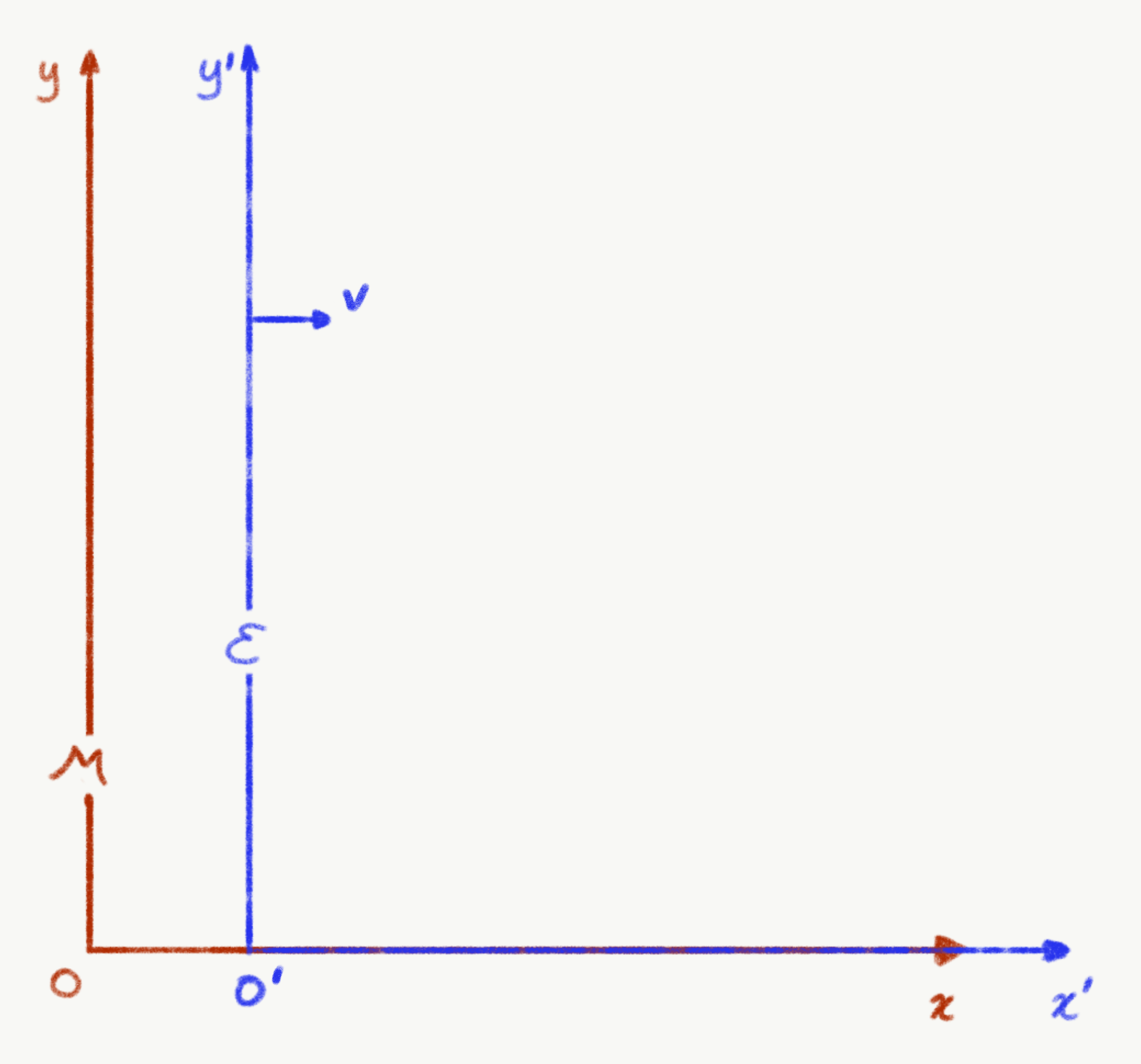
In frame \(\mathcal{M}\), the displacement of the origin of \(\mathcal{E}\) after elapsed time \(\Delta t\) is given by the law of uniform motion:
\[ \Delta x = v \Delta t \tag{3}\]
From Albert’s perspective inside his car, he remains at rest at his own origin: \(v' = 0\), so \(\Delta x' = 0\).
Invariances
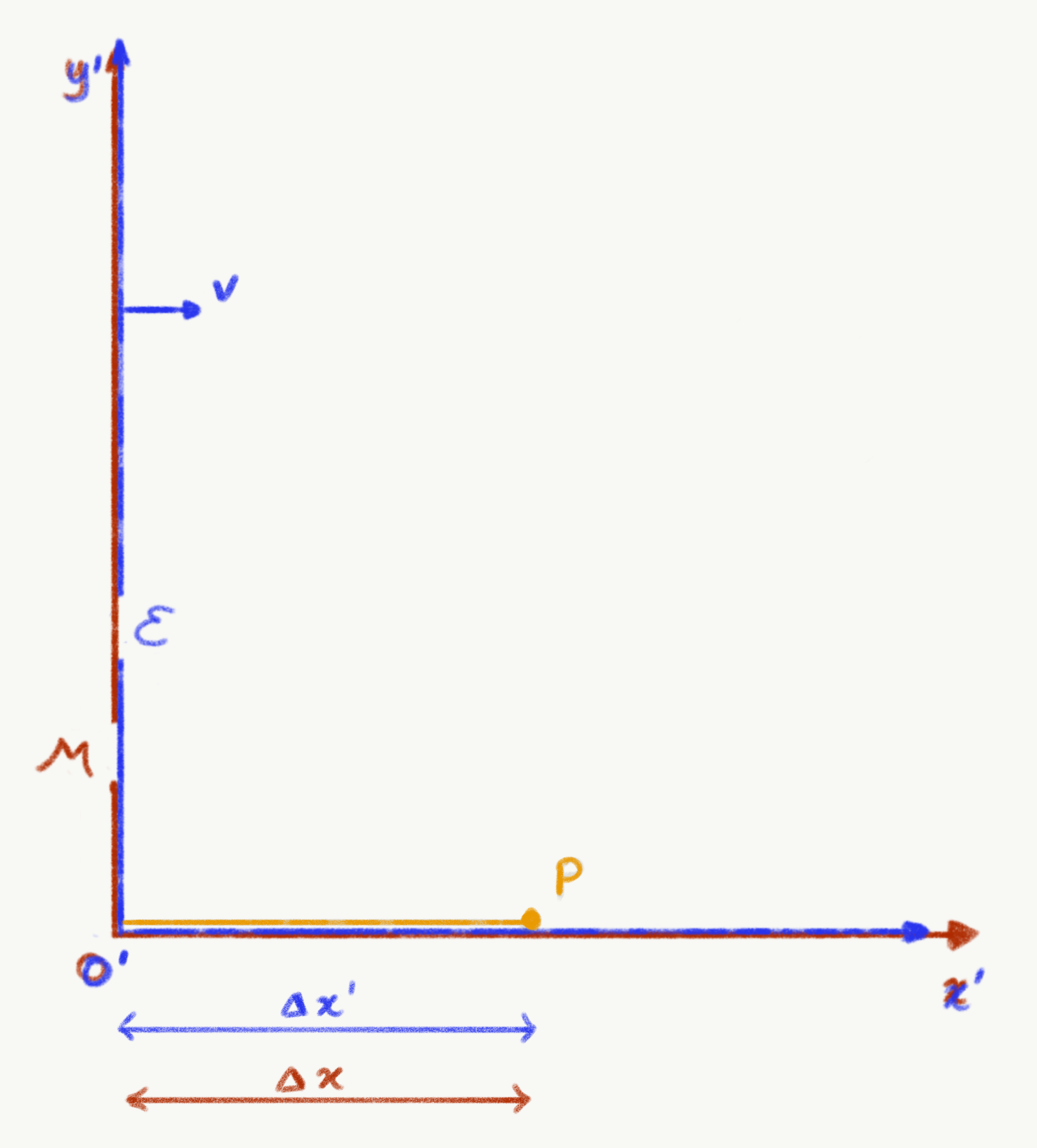
Suppose that at the synchronised instant \(t = t' = 0\), Albert fires a photon \(P\) along the positive \(x\)-axis (Figure 2). Because transverse coordinates do not change (\(y = y' = 0\) and \(z = z' = 0\)), we focus purely on \((x, t)\) and \((x', t')\).
By Einstein’s second postulate of special relativity, the speed of light \(c\) is identical in all inertial reference frames. Therefore, the distance traversed by photon \(P\) satisfies:
\[\Delta x' = c\Delta t', \qquad \Delta x = c\Delta t.\]
Squaring both relations to ensure positive definite quantities and rearranging:
\[(\Delta x')^2 - (c\Delta t')^2 = 0,\]
\[(\Delta x)^2 - (c\Delta t)^2 = 0.\]
Equating both expressions yields:
\[ (\Delta x')^2 - (c\Delta t')^2 = (\Delta x)^2 - (c\Delta t)^2 \tag{4}\]
Even though observers in \(\mathcal{M}\) and \(\mathcal{E}\) assign different spatial and temporal coordinates to event \(P\), both agree precisely on the value of \((\Delta x)^2 - (c\Delta t)^2\). This quantity is invariant.
Wick rotation and imaginary time
Number sets and geometric transformations
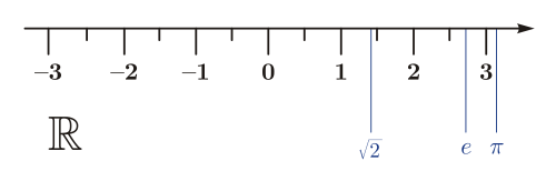
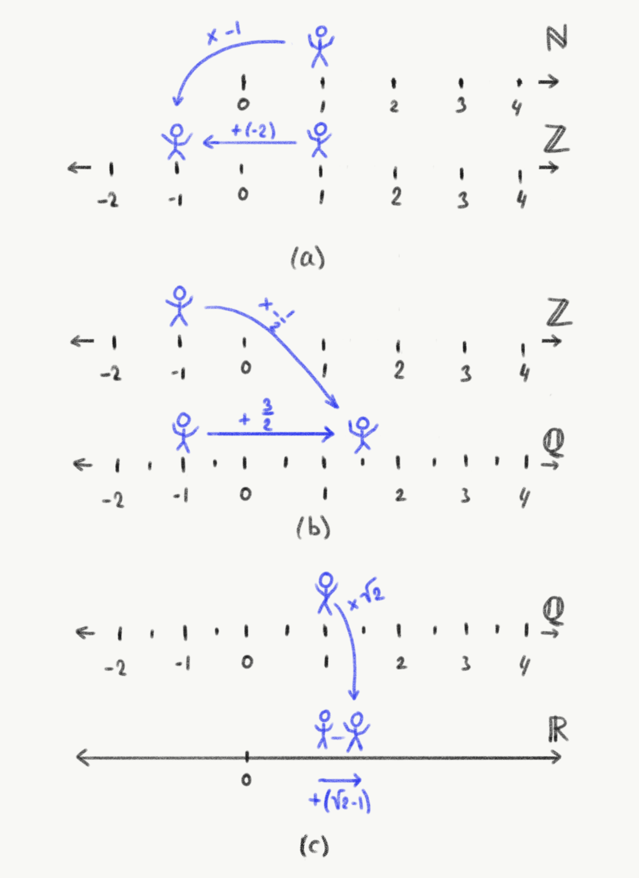
Historically, number systems expanded from counting numbers \(\mathbb{N}\) to integers \(\mathbb{Z}\), rational numbers \(\mathbb{Q}\), and the real continuum \(\mathbb{R}\) (Figure 3). Moving between these sets corresponds to one-dimensional translations along the line (Figure 4).
In the sixteenth century, solving polynomial equations necessitated introducing the imaginary unit \(i = \sqrt{-1}\). Extending the real line orthogonally with an imaginary axis formed the complex plane \(\mathbb{C}\).
Crucially, multiplying a real number by \(i\) does not represent a translation: it corresponds to a quarter-turn rotation of \(\pi/2\) (\(90^\circ\)) in the complex plane (Figure 5).
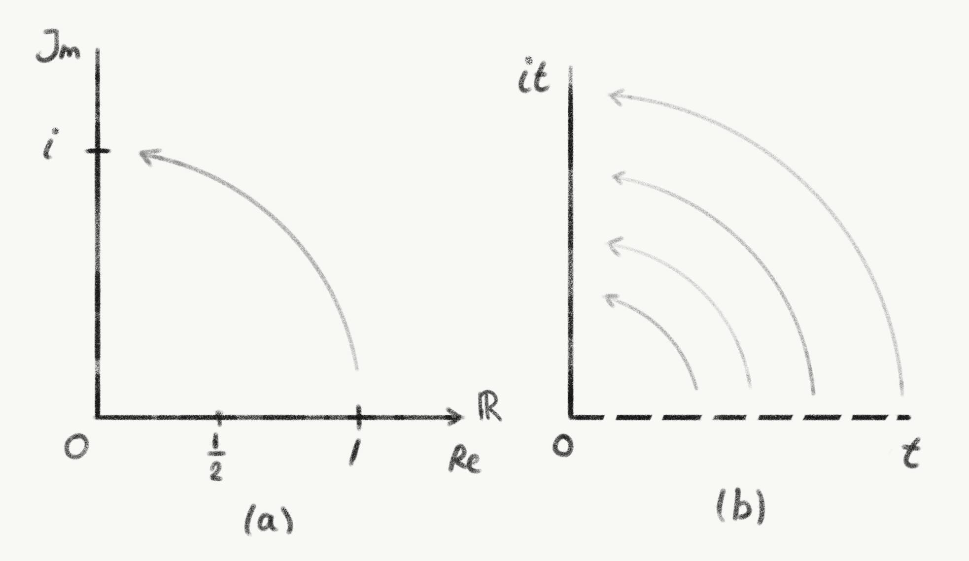
Multiplying the entire temporal coordinate by \(i\) transforms real time into imaginary time: \(t \mapsto it\). This mathematical operation is termed a Wick rotation.
Spacetime diagrams and units
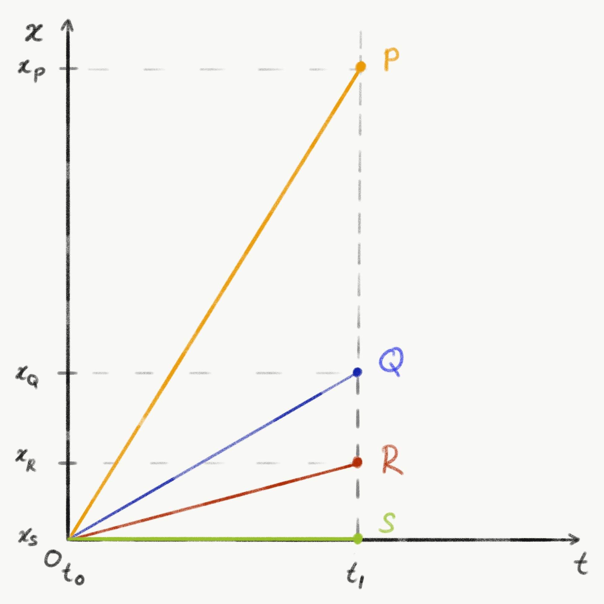
In introductory physics, distance is typically plotted on the vertical axis and time on the horizontal axis (Figure 6). Relativistic physics reverses this convention, placing distance \(x\) on the horizontal axis and time \(t\) on the vertical axis (Figure 7).
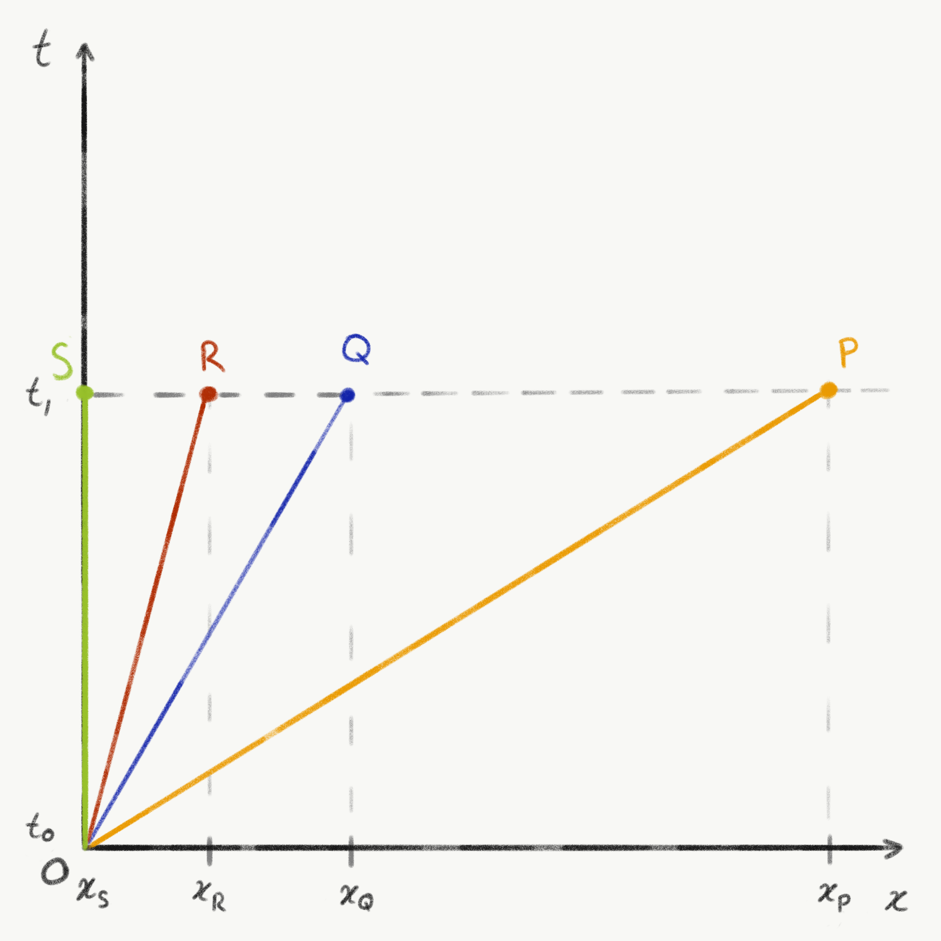
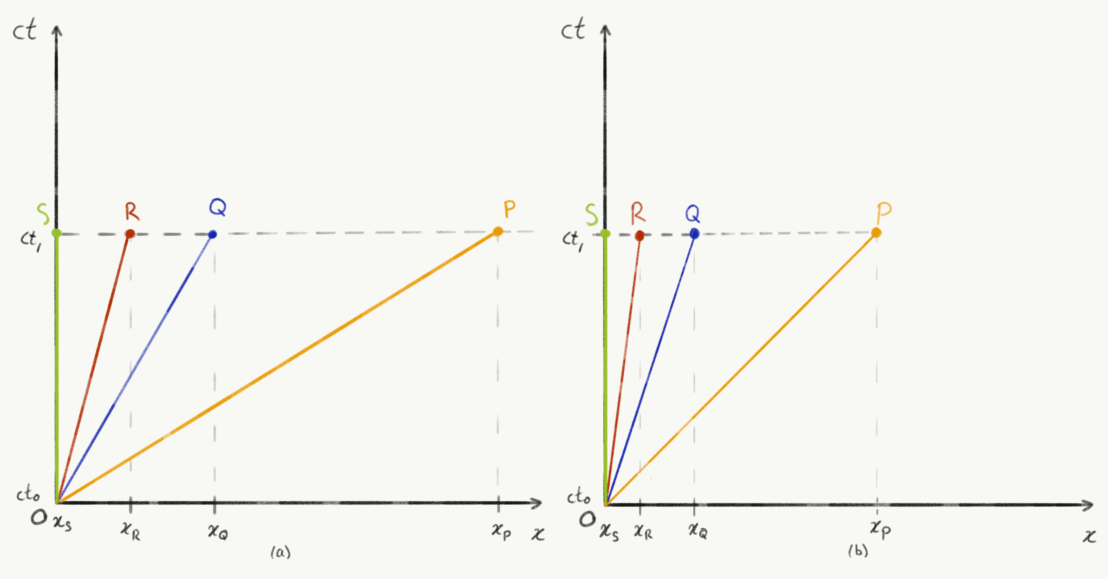
Because spatial distance (metres) and time (seconds) carry different dimensions, we scale time by the constant speed of light: \(t \mapsto ct\). Setting \(c = 1\) in natural units orientates the worldline of light at an angle of \(\pi/4\) (\(45^\circ\)) with respect to the coordinate axes (Figure 8).
Wick rotation to imaginary distance
Applying a Wick rotation to the scaled coordinate \(ct\) yields an imaginary temporal coordinate:
\[ct \longmapsto ict.\]
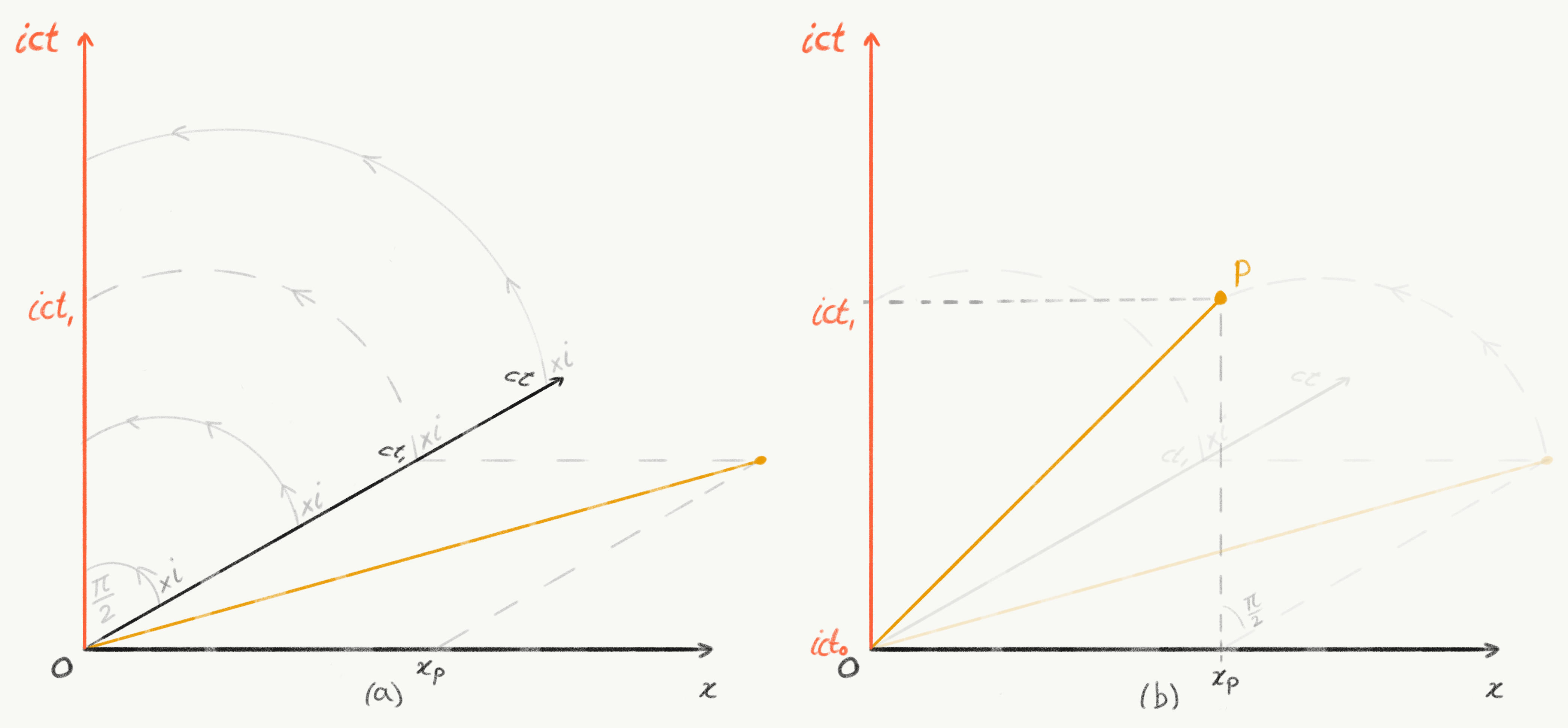
As shown in Figure 9, this operation rotates the temporal axis by \(\pi/2\) into the complex plane, carrying the worldlines along with it.
Deriving the Lorentz transformations
Invariant worldlines in Euclidean complex space
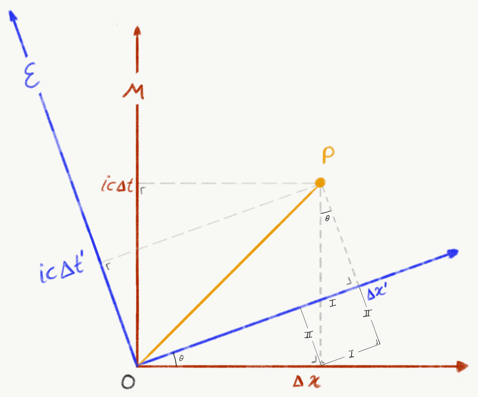
In the complex coordinate plane \((x, ict)\), the squared distance from the origin to event \(P\) is evaluated using the standard Pythagorean metric (Figure 10):
\[(OP)^2 = (\Delta x)^2 + (ic\Delta t)^2 = (\Delta x')^2 + (ic\Delta t')^2.\]
Because \(i^2 = -1\), this identity simplifies directly to:
\[(\Delta x)^2 - c^2(\Delta t)^2 = (\Delta x')^2 - c^2(\Delta t')^2.\]
Through imaginary time, the hyperbolic spacetime interval of special relativity becomes an ordinary Euclidean distance invariant under planar rotations.
Coordinate projections
From the geometry of Figure 10, the primed coordinates in frame \(\mathcal{E}\) are related to the unprimed coordinates in \(\mathcal{M}\) by a rotation of angle \(\theta\):
\[\Delta x' = \Delta x\cos\theta + \text{I}, \qquad \text{where } \text{I} = ic\Delta t\sin\theta,\]
\[ \Delta x' = \Delta x\cos\theta + ic\Delta t\sin\theta \tag{5}\]
\[ic\Delta t' = ic\Delta t\cos\theta - \text{II}, \qquad \text{where } \text{II} = \Delta x\sin\theta,\]
\[ ic\Delta t' = ic\Delta t\cos\theta - \Delta x\sin\theta \tag{6}\]
To relate rotation angle \(\theta\) to relative velocity \(v\), consider the origin \(O'\) of frame \(\mathcal{E}\). Because Albert remains at rest at his own origin, \(\Delta x' = 0\). Substituting this condition into Equation 5:
\[\Delta x\cos\theta + ic\Delta t\sin\theta = 0.\]
Rearranging:
\[\dfrac{\sin\theta}{\cos\theta} = \tan\theta = -\dfrac{\Delta x}{ic\Delta t} = -\dfrac{v}{ic}.\]
Multiplying numerator and denominator by \(i\) (recalling \(i^2 = -1\)):
\[ \tan\theta = \dfrac{iv}{c} \tag{7}\]
Constructing the trigonometric relations
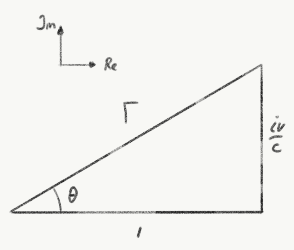
Writing \(\tan\theta = \dfrac{iv/c}{1}\) corresponds to a right triangle with adjacent side 1 and opposite side \(iv/c\) (Figure 11). The hypotenuse \(\Gamma\) is found via the Pythagorean theorem:
\[\Gamma^2 = 1^2 + \left(\dfrac{iv}{c}\right)^2 = 1 - \dfrac{v^2}{c^2} \implies \Gamma = \sqrt{1 - \dfrac{v^2}{c^2}}.\]
The sine and cosine of the complex rotation angle are therefore:
\[\cos\theta = \dfrac{1}{\Gamma} = \dfrac{1}{\sqrt{1 - v^2/c^2}},\]
\[\sin\theta = \dfrac{iv/c}{\Gamma} = \dfrac{iv/c}{\sqrt{1 - v^2/c^2}}.\]
Assembling the transformation equations
Substituting \(\cos\theta\) and \(\sin\theta\) into the spatial projection Equation 5:
\[\Delta x' = \Delta x \left(\dfrac{1}{\sqrt{1 - v^2/c^2}}\right) + ic\Delta t \left(\dfrac{iv/c}{\sqrt{1 - v^2/c^2}}\right).\]
Since \(i \cdot i = -1\):
\[\Delta x' = \dfrac{\Delta x - v\Delta t}{\sqrt{1 - v^2/c^2}}.\]
Measuring coordinates directly from the shared origin (\(x_0 = t_0 = 0\)), this recovers the spatial Lorentz transformation:
\[x' = \dfrac{x - vt}{\sqrt{1 - v^2/c^2}}.\]
Next, substituting into the temporal projection Equation 6:
\[ic\Delta t' = ic\Delta t \left(\dfrac{1}{\sqrt{1 - v^2/c^2}}\right) - \Delta x \left(\dfrac{iv/c}{\sqrt{1 - v^2/c^2}}\right).\]
Dividing the entire equation by the common factor \(ic\):
\[\Delta t' = \dfrac{\Delta t - (v/c^2)\Delta x}{\sqrt{1 - v^2/c^2}}.\]
Expressed in coordinate form, this yields the relativistic time transformation:
\[t' = \dfrac{t - vx/c^2}{\sqrt{1 - v^2/c^2}}.\]
Setting \(\beta = v/c\) and \(\gamma = 1/\sqrt{1 - \beta^2}\), the full set of Lorentz transformations in standard four-vector notation is:
\[\begin{aligned} ct' &= \gamma(ct - \beta x), \\ x' &= \gamma(x - \beta ct), \\ y' &= y, \\ z' &= z. \end{aligned}\]
Through the elegance of Wick rotation, the Lorentz boost of special relativity is revealed to be nothing other than a rotation in Euclidean spacetime with an imaginary time axis.
Image credits and references
- Featured image: Ruler scales texture by arielrobin via Pixabay (CC0 Public Domain).[cite: 63]
- Spacetime diagrams, Minkowski projections, and complex geometric triangles by KJ Runia.
- Hawking, S. (2001). The Universe in a Nutshell. New York: Bantam Books.
- Poincaré, H. (1906). “Sur la dynamique de l’électron”, Rendiconti del Circolo Matematico di Palermo.
- Einstein, A. (1905). “Zur Elektrodynamik bewegter Körper”, Annalen der Physik, 322(10), pp. 891–921.
- Wick, G. C. (1954). “Properties of Bethe-Salpeter Wave Functions”, Physical Review, 96(4), pp. 1124–1134.